One of the core tasks in information retrieval is searching. Anyone who deals with large amounts of text data (and that’s almost all of us) knows how difficult this seemingly simple task can be. If your search term is too broad, you may find yourself sifting through an impossible quantity of documents. And if your search term is too narrow, you could be missing out on relevant results. So how do we decide which documents are the most relevant to our search?

Search relevance is a difficult problem—and modern search engines employ highly sophisticated (and proprietary) algorithms to deal with the issue. We won’t delve into those algorithms, but let’s look at some simple strategies that you might employ in your own information retrieval applications.

State of the Union

As a sample dataset, we will be exploring the text of State of the Union (SotU) addresses by U.S. Presidents. Imagine that you’re a historian studying different policy priorities in U.S. history. How would you decide which SotU address was most related to your topic of interest? For example, say you are interested in taxes. Is a simple search in the corpus for “taxes” enough? Will that lead to too many results and information overload? Let’s find out!

Exploring the Data

Our dataset consists of text documents, which we have loaded along with metadata into a Pandas dataframe for easy manipulation. As per usual, the first step is looking at our data to understand its shape and contents.

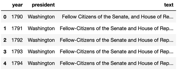
In looking at the first few rows of our data, we can see that it contains year, president, and text columns. In total, there are 228 rows, representing different SotU speeches, and covering a timeframe from 1790 to 2018.

Simple Search

Now that we have our data, let’s start searching for specific terms. At its most basic, a search query asks the question “which documents contain all of the terms in this query?” This is a simple strategy and we can use it to search through the text column of our dataframe.

Putting on our historian hat, let’s imagine that we are interested in comparing technology and tax policy. As part of our work, we want to find all of the SotU addresses that discuss both issues. To do this, we will use the search query “technology taxes”. For the sake of simplicity, we will treat this as a boolean query in the form “technology AND taxes”.

First, we will need to split our query into individual search terms and then filter our dataframe for all of the observations where the text column has at least one occurrence of each of the terms in our query. Let’s write a function to carry out this search.

def search_df_texts(df, query_string: str):
    """
    - Parameters: df (Pandas DataFrame), query_string (string). df must 
      contain a "text" column.
    - Returns: A subset of df containing only rows where each term in 
      query_string appeared as a substring in df["text"].
    """
    terms = query_string.lower().split(" ")
    filters = [df["text"].str.lower().str.contains(term) for term in terms]
    return df[np.all(filters, axis=0)]

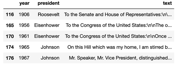
If we use this method to search our dataframe with the query "technology taxes", we get 38 results, the top five of which are:

Certainly this is a useful query—we have cut 228 documents down to 38, but how do we know where to start? Our dataframe was already sorted in chronological order, which is also how the search results are sorted. However, this tells us nothing about which of the SotU speeches is most relevant to our search. We’re going to have to read through all 38 speeches to see which ones are the most useful. Surely there must be a better way!

Bag-of-Words and the Term-Document Matrix

To improve on our simple search model, we need some kind of metric to use when comparing search results. We already know that all of the results contain each of our search terms at least once, so what else can we do? The obvious solution is to look at word frequency. If one document contains our search terms many times, and another document just a few times, then the first one is likely more relevant.

To look at word frequency, we can use the so-called bag-of-words (BoW) model. A BoW turns a document into a collection of token-frequency tuples. We can view this collection as a vectorized version of our text, which is useful in various machine learning tasks. For our purposes though, we aren’t feeding the model into an algorithm—rather, we want to use it as a metric when comparing search results.

To use the BoW as a search relevance metric, we can convert it into a term-document matrix, which is a table where each row is a document and each column is a token. The values in the cells are the number of times a particular token occurs in each document. Using this, we can sort our search results by the count of a particular token (or the sum of the counts of all the terms in our search).

Data Preparation

To get started, we will need to tokenize our documents and build a vocabulary from the overall collection. A vocabulary is the set of unique tokens in our text and will be used as the columns in our term-document matrix. To carry out these tasks, we can use spaCy for tokenization and Gensim to build a vocabulary (aka dictionary).

# load spaCy model
nlp = spacy.load("en_core_web_md")

# tokenize documents
def spacy_doc(model, text, lower=True):
    """
    - Parameters: model (spaCy model), text (string), lower (bool).
    - Returns: A spaCy Document object processed using the provided
      model. Document is all lowercase if lower is True.
    """
    if lower:
        text = text.lower()
    return model(text)

sotu_docs = [spacy_doc(nlp, text) for text in sotu_df["text"]]

# build dictionary
def get_token_texts(doc):
    """
    - Parameters: doc (spaCy Document object).
    - Returns: A list of strings based on the text value of each token
      in doc.
    """
    token_list = [token for token in doc]
    return [token.text for token in token_list]

def build_dictionary(doc_list):
    """
    - Parameters: doc_list (list of spaCy Document objects).
    - Returns: A Gensim Dictionary, built using the tokens in each
      document contained in doc_list.
    """
    return Dictionary([get_token_texts(doc) for doc in doc_list])

sotu_dictionary = build_dictionary(sotu_docs)

Building a Term-Document Matrix

Now that we have our tokenized documents and our corpus vocabulary, we can build our BoW representations for each text and use those to create term-document matrices. Of note, Gensim Dictionary objects represent each token by a numerical id rather than the token text. Since we’re interested in manually inspecting our term-document matrices, we should re-label the columns with the actual token texts and convert the matrix into a dataframe for easy manipulation.

def build_corpus(doc_list, dictionary):
    """
    - Parameters: doc_list (list of spaCy Document objects), dictionary
      (Gensim Dictionary object).
    - Returns: A list of documents in bag-of-words format, containing
      tuples with (token_id, token_count) for each token in the text.
    """
    return [dictionary.doc2bow(get_token_texts(doc)) for doc in doc_list]

def build_td_matrix(doc_list, dictionary):
    """
    - Parameters: doc_list (list of spaCy Document objects), dictionary
      (Gensim Dictionary object).
    - Returns: A term-document matrix in the form of a 2D NumPy Array,
      where each row contains the count of a token in the corresponding
      document and each column index is the id of a token in the
      dictionary.
    """
    corpus = build_corpus(sotu_docs, sotu_dictionary)
    tdm = []
    for bow in corpus:
        vector = np.zeros(len(dictionary))
        for token_id, token_count in bow:
            vector[token_id] = token_count
        tdm.append(vector)
    return np.array(tdm)

def build_term_document_df(doc_list, dictionary):
    """
    - Parameters: doc_list (list of spaCy Document objects), dictionary
      (Gensim Dictionary object).
    - Returns a term-document matrix in the form of a Pandas Dataframe, 
      where each row is a document and each column is a token. Values in
      the dataframe are token counts for the given document / token.
    """
    tdm = build_td_matrix(doc_list, dictionary)
    cols = list(dictionary.token2id.keys())
    return pd.DataFrame(tdm, columns=cols, dtype=pd.Int64Dtype)

sotu_td_df = build_term_document_df(sotu_docs, sotu_dictionary)

Exploring the Term-Document Matrix

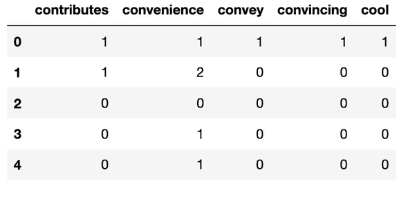
At this stage we have a list of tokenized documents, a corresponding vocabulary, and a term-document matrix stored in a dataframe as sotu_td_df. This dataframe has the same number of observations (documents) as our original sotu_df dataframe, except it has 28,393 columns, each of which represents a different token in the vocabulary. The dataframe is far too large to look at the whole thing, but we can get an idea by looking at a subset.

Each entry in our dataframe contains the frequency count for a given token in a document. Note that this is a sparse matrix, meaning that the vast majority of entries are zero (because most SotU speeches will not use every word in the vocabulary—otherwise they would very long speeches!)

It’s important to note that the row indices of sotu_td_df match indices in our sotu_df dataframe, which contains the text and metadata about each SotU speech. We had better not change the indices otherwise we won’t be able to join them later!

Searching a Term-Document Matrix

It looks like we’re in good shape. Now that we have a term-document matrix and we have a metric that we can use when assessing search relevance. We will still filter our sotu_df dataframe for those rows that contain our search terms in the text column, except now we can join the dataframe with the term frequency counts from sotu_td_df and sort accordingly. Let’s see what happens with our earlier query of "technology taxes" using the following search function.

def search_td_df(td_df, text_df, query_string: str):
    """
    - Parameters: td_df (Pandas DataFrame) representing a term-document
      matrix, text_df (Pandas DataFrame) with a "text" column and rows 
      that correspond to the td_df, and query_string (string).
    - Returns: A new dataframe that only contains rows from text_df where
      the "text" column had at least one occurence of each term in
      query_string. Additional columns are added to show the count of
      each term and the total count of all terms.
    """
    terms = query_string.lower().split(" ")
    filters = [td_df[term] > 0 for term in terms]
    filtered_td_df = td_df[np.all(filters, axis=0)][terms]
    filtered_td_df["terms_sum"] = filtered_td_df.agg(sum, axis=1) \
        .astype("int64")
    full_df = text_df.merge(filtered_td_df, 
        left_index=True, right_index=True)

    return full_df.sort_values("terms_sum", ascending=False)

Once again we get back 38 results, except this time they are sorted in a more meaningful order.

Already we can see that searching our term-document matrix produced more interesting results than our simple search. We can see term counts for each of our query terms as well as a sum of all the counts together. Given that “technology” and “taxes” are mentioned more frequently in the documents at the top, those documents are probably a good place to start.

Of course, there are more nuanced ways to look at the search relevance problem. To finish up our introduction to search relevance, we’ll look at one more model.

Term Frequency-Inverse Document Frequency

Term frequency alone is a reasonable metric for search relevance, but imagine a case where you are searching for a term that is relatively common across the entire set of documents. Perhaps the term “government” or “america” in the case of our corpus of SotU addresses. Nearly all of the documents are likely to mention such search terms. Some may use the word “government” more often than others, but because of how common the term is across all the documents, it starts to lose its meaning.

One way of addressing this problem is the term frequency-inverse document frequency (TF-IDF) model. Rather than use term frequency as our metric, we can use TF-IDF to give more weight to rare terms over common terms. We do this by calculating the document frequency (the number of documents that include a term at least once, denoted $dft$) and the inverse document frequency (calculated as $log\left(N/dft\right)$, where $N$ is the total number of documents) and then multiplying it by the term frequency.

The result is a measure that still takes into account the number of times a term appears in a document, but gives priority to those terms that are generally rare. Let’s take a look at TF-IDF in action, starting by converting our term-document matrix values into TF-IDF values.

def document_frequency(td_df, term: str):
    """
    - Parameters: td_df (Pandas DataFrame) representing a term-document
      matrix, and term (string).
    - Returns: The document frequency value showing the number of
      documents in td_df where term occurs at least once.
    """
    return td_df[td_df[term] > 0].shape[0]

def inverse_document_frequency(td_df, term: str):
    """
    - Parameters: td_df (Pandas DataFrame) representing a term-document
      matrix, and term (string).
    - Returns: The inverse document frequency value for term, calculated
      as N / log(dft) where N is the number of documents in td_df and
      dft is the document frequency value for term.
    """
    N = td_df.shape[0]
    dft = document_frequency(td_df, term)
    return (N / np.log10(dft))
    
def build_tfidf_df(td_df):
    """
    - Parameters: td_df (Pandas DataFrame) representing a term-document
      matrix.
    - Returns: Returns a term frequency-inverse document frequency
      (TF-IDF) matrix in the form of a Pandas DataFrame, where each row
      is a document and each column is a token. Values in the dataframe
      are TF-IDF values for the given document / token.
    """
    def calculate_tfidf(col, td_df):
        idf = inverse_document_frequency(td_df, col.name)
        return col * idf
    
    return td_df.apply(calculate_tfidf, td_df=td_df)

sotu_tfidf_df = build_tfidf_df(sotu_td_df)

Exploring the TF-IDF Matrix

Before looking at the TF-IDF matrix, let’s see how some IDF scores compare for a relatively common word in the corpus like “government” and a rare one like “moon”. By applying the aforementioned TF-IDF formula, we see that “government” appears in 227 out of 228 documents and has an IDF score of 96.77. In contrast, “moon” appears in only 12 out of 228 documents and has an IDF score of 211.27. In other words, “government” is very common and “moon” is quite rare. This means that if we used the query "government moon" to search our TF-IDF matrix, appearances of the term “moon” would carry more than twice as much weight as appearances of the term “government”.

Similarly, if we look at our previous query of "technology taxes", we can see that “technology” appears in 50 out of 228 documents and has an IDF score of 134.20 and “taxes” appears in 131 out of 228 documents and has an IDF score of 107.66. How will this affect our search order?

Searching the TF-IDF Matrix

Once again, let’s put our query into a search function—this time using the TF-IDF matrix.

def search_tfidf_df(tfidf_df, text_df, query_string: str):
    """
    - Parameters: tfidf_df (Pandas DataFrame) representing a tf-idf
      matrix, text_df (Pandas DataFrame) with a "text" column and rows
      that correspond to the tfidf_df, and query_string (string).
    - Returns: A new dataframe that only contains rows from text_df where
      the corresponding tf-idf value was greater than zero for each of
      the terms in query_string. Additional columns are added to show the
      tf-idf value for each term and the sum of the tf-idf values. 
    """
    terms = query_string.lower().split(" ")
    filters = [tfidf_df[term] > 0 for term in terms]
    filtered_tfidf_df = tfidf_df[np.all(filters, axis=0)][terms]
    filtered_tfidf_df["tfidf_sum"] = filtered_tfidf_df.agg(sum, axis=1)
    full_df = text_df.merge(filtered_tfidf_df, 
                            left_index=True, right_index=True)

    return full_df.sort_values("tfidf_sum", ascending=False)

As expected, we get back 38 results, but you will notice that the order is once again different!

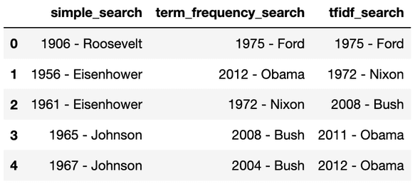
In our TF-IDF model, the word “technology” carried about 25% more weight than the word “taxes”. And indeed, it seems to have affected the results. The rank order of the top five results from the three searches is as follows.

The results between the term frequency and TF-IDF searches may not seem all that different—but imagine that you are working with a significantly larger data set. Weighting your search with TF-IDF may prove decisive in your effort to find the most relevant search results.

Challenges

Our goal in comparing simple searches, term frequency searches, and TF-IDF searches isn’t necessarily to determine which is best. Rather, the goal has been to see how different methods of information retrieval produce different results. Which model you use will depend in part on your goals.

Of course, our basic introduction ignores a lot of important issues. For example, should term proximity matter? Should we only return results that include all search terms (as we chose to do here) or should we also return results for partial matches? What about related words? Should a search for “taxes” also return results for “tax” and “taxation”? Or perhaps we shouldn’t focus on words at all, but instead focus on themes. Perhaps a search for “technology” should also return documents that discuss “innovation” and “science”. The list of possible refinements goes on.

Search relevance, and information retrieval more broadly, is a complex and fascinating topic. Hopefully this has been an interesting introduction. Stay tuned for more articles on how to explore your text data sets!